29. Semilandmarks and Surfaces
We’ve spent a considerable time talking about semilandmarks, but that’s because — as I hope you’ll agree by now — they are by far the most intuitive and useful of morphometric objects. Landmarks arguably do have more biological information content, at least in a theoretical sense. However in many, if not most, practical contexts you’re simply not going to have the information you need to specify the location of a sufficient number of true landmarks to, or be able to locate these landmarks in places that, enable you to test the hypotheses you’re interested in across all specimens in your sample. In such all-too-common cases, the ability to employ sets of semilandmarks as descriptors of morphological variation can make the difference between being able to apply a quantitative approach to morphological analysis or being forced to rely on qualitative, observation-based assessments. In the last two essays of this series we’re going to push semilandmarks to the very limits of their utility. This will allow me to end this column, in a curious manner, back where I started it ten years ago with a consideration of what it means to ‘observe, morphology and how we might use mathematical tools to inform, supplement, and extend our qualitative observations.
You also might have wondered why I’ve spent so much time on two-dimensional (2D; x,y) morphometric analysis when, increasingly, three-dimensional (3D; x,y,z) analyses are becoming the standard. There are several reasons. Historically the methods and procedures — even shape theory — was worked out for the 2D case first. The methods I’ve described to this point have been discussed in the context in which they were first presented to the scientific community. Granted, in many cases extension of these procedures to the third dimension required few, if any, modifications. Nevertheless, morphometrics has been developed and pursued in the context of 2D representations of form far long than in the context of 3D data and, at the moment, 2D morphometric investigations outnumber 3D investigations by a considerable margin. Of course, this dimensional priority pertains only to the data we collect from organismal bodies. Morphometric data analysts have utilized higher dimensional representations of form/shape similarity/difference for a very long time, even though this distinction often seems to be forgotten (or ignored) in many published technical reports.
This historical focus on 2D data did not derive from any failure to appreciate the 3D character of organismal morphology. Despite the fact that quantitative morphologists have almost always described and discussed their results as if the 2D (apparent) representation of 3D forms was a matter of so little consequence it was scarcely worth mentioning, most experienced practitioners of the morphometric arts were acutely aware of the limitations representation of 3D objects with 2D data imposed on their investigations. Our collective silence on this topic was more one of embarrassment than evasion. The simple fact was that all but a very few of us did not have access to 3D digitizers and 3D data processing software throughout the 1980s and 1990s. This began to change in the late 1990s with the advent of reasonably low cost, 3D physical, acoustic, and (finally) optical digitizers. Now, the situation has changed to such an extent that PhD student visitors to The Natural History Museum (London) often to turn up with carrying large cases containing an amazing variety of 3D digitizers that they have the inestimable pleasure of lugging across Europe — sometimes across the world — on their ‘museum visitation’ data-collection trips.
Once these 3D digitizers had appeared on the market, or more to the point, in the hands of morphometricians, it was not long before 3D landmark and (even) 3D outline analyses began to be published. In most cases the procedures involved in the analysis of landmark and outline configurations were able to be extended to encompass the 3D case rather easily. Nevertheless, while this proved both a welcome and easily achieved technical advance that unquestionably enhanced the appropriateness and sensitivity of the hypotheses tests to which these new 3D data were applied, by themselves these extensions did not achieve what many of us really wanted; a morphometric method that was capable of accurately representing and analyzing 3D surfaces.
The problem with surfaces is obvious once you stop and think about it. Surfaces contain a wealth of morphological detail that systematists and taxonomists make use of routinely. But they often don’t exhibit many landmarks or outlines. For example, take these three fossil representatives of the bivalve genus Astarte collected from the Red Crag Formation in the UK.
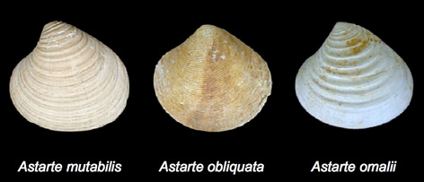
Figure 1. Three Pleistocene fossil bivalve species from the Red Crag Formation, Essex, UK.
In plan view each shell has at least one obvious landmark (the tip of the beak) and each has an outline. But the most important feature(s) distinguishing these species from one another is the character of the valve surface. Astarte mutabilis is characterized by a somewhat smooth but irregularly spaced series of annular growth rings set on a highly vaulted surface. Astarte obliquata displays a much lower valve vault on which a more regular series of fine annular growth rings are set, each with distinctly and regularly rounded ridges and furrows. And Astarte omalii is characterised by a valve vault that is even more pronounced than that of A. mutabilis, but whose surface is typified by a prominent smooth and coarsely undulating annular ornament. Qualitative descriptions like these are fine for explaining how someone might separate these three specimens by observational criteria alone. But how can we use morphometrics to characterize these surfaces so that we might introduce a degree of quantitative rigour to the morphological analysis of these surfaces?
Clearly, landmarks are out as a reasonable quantitative form-description strategy. These forms could be represented by outlines. If we wanted to test some hypothesis that was captured adequately by the outline (e.g., shape of the valve opening) outlines would be just the ticket. But as a proxy for the general character of morphological similarity and difference the outline is only one bit of a much larger puzzle; and with regard to these particular shells, a pretty nondescript bit at that. The outlines of A. mutabilis and A. omalii are broadly similar to each other and differ from A. obliquata. However, from the standpoint of the valve morphology enclosed by their outlines, these three species could hardly be more different. Therefore, using differences between the form or shape of these shells’ outlines as an index of general form/shape similarity would result in a badly biased representation of their true similarity. If we opted instead for making inter-specimen comparisons based on landmarks this bias grows even worse!
There is a wealth of morphological information encoded in the surfaces of these bivalve shells. Qualitative taxonomists have access to this information and use it as a matter of course to make distinctions between these species. But very little of this information is such that it can be represented by a small set of landmark point positions or strings of outline semilandmarks. What do to?
The first step in solving this problem is to decide what is needed. If we could represent the surfaces of these valves in a manner consistent with the use of geometric morphometrics, what would that look like? As the sine qua non of geometric morphometric analysis is the mathematical point, if we could scatter mathematical points over the surfaces of these valves, and then match them in some way across the different specimens in the sample, we’d be able to create a valid index of form/shape similarity and difference using the standard geometric morphometric toolbox. Let’s try that.
With the advent of those digitizers I was talking about, scattering mathematical points across the surfaces of the values is easier than you might think. Figure 2 shows the results of fairly low-resolution 3D scans of the Astarte specimens shown in Figure 1. These point clouds are formed out of 5,528, 6,571 and 5,614 points for A. mutabilis, A. obliquata, and A. omalii respectively.
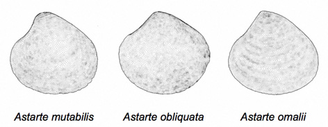
Figure 2. Digitized points of the surface of the three Astarte specimens.
As you can see, the point spacing achieved by these low-resolution scans is more than sufficient to represent the gross morphology of the valve surfaces as well as a considerable amount of surface detail. Unfortunately, these point clouds cannot be compared in the manner sets of landmarks and strings of semilandmarks can. First, different specimens are represented by different numbers of points. Second, individual points in each point-cloud dataset have no necessary geometric or biological correspondence to points at same position in the sequences of other point-cloud datasets. As a consequence, even if we could constrain each point-cloud dataset to contain the same number of points — a task that can be accomplished easily in software — this lack of geometric or biological correspondence would still prevent us from using the raw point-cloud coordinates as meaningful morphological descriptors from the standpoint of quantitative form/shape comparison.
In addition there is an information redundancy issue in these data. Even at these rather modest levels of spatial resolution there is a considerable amount of geometric autocorrelation in the datafiles representing these valve surfaces. The values of neighbouring points tend to be very similar, and so not to contribute much new information either to the representation of individual forms/shapes or to their comparison with one another. Ideally we’d like to reduce this redundancy prior to analysis in order to increase analytic efficiency by reducing extraneous computational overhead.
Somehow we need to use these data as the basis for the specification of a surface point-sampling scheme that will deliver sequences of (semilandmark) points that bear a consistent geometric correspondence both to one another and to the underlying morphology. There are a number of ways to approach this problem. One of the most straightforward and flexible is a sampling technique I call eigensurface analysis.
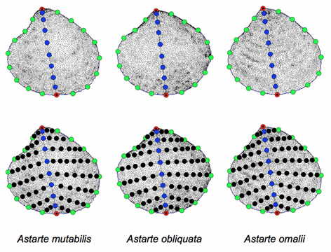
Figure 3. Steps in sampling surface morphology using the eigensurface procedure as applied to the three Astarte specimens. The red symbols mark positions of the landmarks used to orient the semilandmark sampling grid, greed symbols the outline semilandmarks, blue the midline semilandmarks, and black the ‘rib’ semilandmarks that join the midline to the outline segments. These are 10-grids in which each half outline and the midline is represented by 10 semilandmarks. Spatial resolution of the sampling network is controlled by increasing or decreasing the number of equally spaced semilandmark points used to represent these dimensions of specimen form. See text for further discussion.
The eigensurface sampling procedure is illustrated in Figure 3. It’s essentially an extension of extended eigenshape analysis (see MacLeod 1999, 2012). Sampling for eigensurface analysis begins with specification of the surface’s outline, which is done in the normal way; with the outline starting at a landmark point (in this case the maximum of curvature represented by the valve’s beak, marked in Figure 3 by a red symbol) and represented as an ordered set of semilandmark coordinates. Each specimen’s outline can be represented by the same number of semilandmark points or different numbers, so long as this number is large enough to accurately represent the form of the outline.
The next step is to select a second landmark that also lies on the form’s outline. This will be used to specify the position of a midline across the surface. In Figure 3 the second landmark is placed at the ventral margin of the valve midway between the two adductor muscle scars (second red symbol located along the lower margin of the drawings comprizing Fig. 3). Obviously, using a constructed point in this manner is a very approximate way of defining the second landmark. It would have been better to have used a more objectively defined and reproducibly located true landmark to tie the path of the midline chord to a well-defined location. But, for these bivalve specimens no more suitable landmark was available. Nevertheless, the marginal midpoint between the two adductor muscles has the highly desirable property of subdividing the valve into two subequal halves and the adductor muscles on which this point’s definition is based are unquestionably homologous (in both the mathematical and biological senses of that term) structures. Once these points have been located sampling of the surface can begin.
Sampling of the specimen’s surface is achieved by using the midline landmarks to subdivide the outline into two segments in the manner of extended eigenshape analysis and interpolating a fixed number of equally spaced semilandmarks along each half-outline segment (the green symbols in Fig. 3). All calculations used in carrying out this interpolation are done using 3D coordinates. As the number of interpolated points chosen for this step effectively sets the resolution of the surface sampling system, this number should be chosen with care, though strategies do exist that will allow the shape complexity of the sample to determine the number of points used to represent the set of surfaces (see MacLeod 1999, 2008, 2012). Next, a chord is drawn that joins the midline landmarks. This chord is projected onto the surface of the specimen (as defined by the point-cloud data), and the same number of equally spaced 3D semilandmarks used to represent the outline half-segments is used (via interpolation) to represent its path across the specimen’s surface (the blue symbols in Fig. 3).
Finally, chords are drawn between each midline semilandmark and the corresponding outline semilandmarks on either side. These chords are projected onto the surface of the specimen and represented via 3D interpolation as a set of equally spaced semilandmarks. For descriptive convenience I’ll refer to the chords joining the midline to the outline as ‘rib’ chords. Since the lengths and shapes of these rib chords will vary across the specimen’s surface, a fixed geometric fidelity index is used to determine how many equally spaced semilandmarks are necessary to represent this chord’s form to a given tolerance criterion (usually 95% of uninterpolated chord 3D length, the black symbols in Fig. 3). Once a preliminary interpolation along each rib has been achieved for each specimen, the number of semilandmarks used to represent each corresponding rib chord in each specimen can be compared across all specimens in the sample and the maximum value used to reinterpolate the geometric representation of that rib. This operation ensures that a minimum standard amount of representational detail is provided in a consistent manner across all specimens in the sample, and that all corresponding ribs across all specimens in the sample are represented by the same number of outline semilandmarks.
The eigensurface sampling procedure results in the creation of a network of semilandmark points that will adapt itself to the 3D form of any shape that is represented by a 3D surface, irrespective of the complexity of that surface, so long as the surface is single valued for all rib chords. To facilitate achievement of a maximally informative fit of the semilandmark system to the underlying form of the specimen, the midline chord can be straight (see Fig. 3) or curved. The only requirement that needs to be respected in deciding on the form of the midline chord is that its path must be able to be specified precisely for each specimen in the sample and it must result in a rib chord network that is single valued for each specimen in the sample. Additionally all surfaces represented by this procedure must be continuous — possess no holes or other missing data.1 Surfaces that fail to meet these criteria can be accommodated in an eigensurface analysis by subdividing them at landmarks into regions, calculating an eigensurface-based network of semilandmark points for each region, and then combining the regional semilandmark networks into a single synthetic dataset for analysis. Similarly, the surfaces of complete, continuous 3D forms can be represented using by using the outline to subdivide the form into ‘upper’ and ‘lower’ halves, using the same set of landmarks and same set of outline data to orient the sampling grid for each half, and combining the two halves into a single synthetic dataset prior to analysis. Note that, if either of these composite form-representation strategies is attempted, care must be taken to eliminate any redundant landmark or outline semilandmark points from the dataset during assembly of the composite data.
As mentioned above, the spatial resolution of an eigensurface sampling network is set by the initial decision of the number of outline and midline semilandmarks to use to represent the form. A lower number (e.g., 10, 20) will sample these surfaces’ gross form, result in the specification of a smaller number of 3D coordinates to submit for analysis, and result in quicker analyses. Higher numbers (e.g., 40, 50) will sample fine details of the surface, result in specification of larger numbers of 3D semilandmarks for analysis, and result in slower, more computation intensive analyses. Of course, the size of the dataset resulting from any particular outline sampling resolution will also be controlled by the geometric complexity of the set of surfaces under investigation as the bulk of the specified semilandmark data comes from the rib semilandmarks.
| Grid Resolution | No. of Semilandmarks | No. of Data Analysis Variables |
|---|---|---|
| 10-Grid | 88 | 264 |
| 15-Grid | 207 | 621 |
| 25-Grid | 493 | 1479 |
| 50-Grid | 2011 | 6033 |
Table 1 provides indicative data for the sizes of the semilandmark datasets that result from different sampling resolutions as applied to 3D scans of the three specimens shown in figures 1 and 2. As can be seen from this table the relation between grid resolution and sampling dataset size is decidedly non-linear. Accordingly, care should be taken in determining how much resolution is necessary to solve the problem, or test the hypothesis, you’re interested in. As with all data analysis problems, not only is it inefficient to collect more data than you need, in many cases doing so introduces other issues into the analytic design (e.g., the need for large sample sizes, see discussion of the Curse of Dimensionality in MacLeod 2007). These issues should be avoided if possible. At the very least large datasets will cause the programmes that implement generalised least-squares (GLS) Procrustes superposition or principal components analysis (PCA) to take an extraordinarily long time to complete their calculations and may well exceed the design limits either of the software or of the computer used to run the software.
Once the eigensurface sampling procedure has produced a set of topologically comparable sets of semilandmark data that quantify geometric variation along the surface of a set of forms, these 3D coordinate data may be submitted to any of the various procedures that make up the geometric morphometric toolkit. Generally speaking this will entail registering these points and transforming them into the Procrustes shape space using GLS Procrustes superposition (Rohlf and Slice 1990, MacLeod 2009a) and using Procrustes PCA (also called relative warps analysis, see MacLeod 2010a) to assess the major trends in shape variation, inspect the ordination of surface shapes in a shape-variance optimised coordinate system, and/or reduce the dimensionality of the data via projection of the shape-coordinate data onto a series of shape variance-optimised, orthogonal, latent vectors (= eigenvectors) as a pre-processing step for additional analyses. One of the most common of these additional analyses will be assessment of the differences between groups in a group-optimized discriminant space using canonical variates analysis (CVA, see Campbell and Atchley 1981, MacLeod 2007). Fortunately, all the shape modelling procedures I’ve discussed in previous essays (see MacLeod 2009b, 2010b) can be used to represent the results of these procedures in a graphical form that greatly enhances our ability to interpret these results and communicate our interpretations to generalized audiences.
In order to illustrate the power of the eigensurface technique I’ve chosen to reanalyze part of the Astarte dataset I used originally to describe it (MacLeod 2008). Plate 1 illustrates the first ten specimens for each of the species-specific datasets.
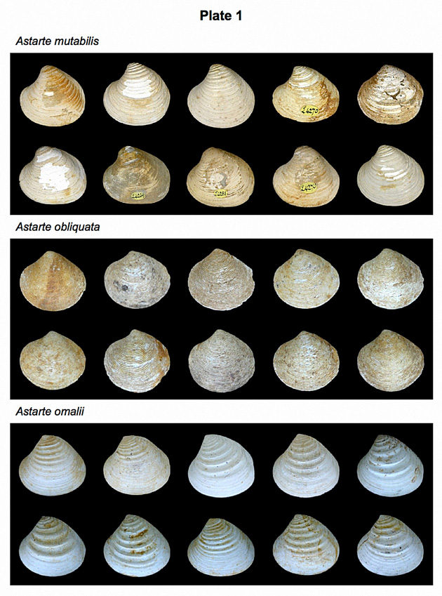
For the purposes of this example the right valves of these specimens were 3D scanned using The Natural History Museum’s Konica-Minolta VIVID 910 laser scanner and the resulting scans processed such that each specimen was represented by 5,000 - 7,000 x,y,z coordinate points. A 15-grid eigensurface sampling resolution was chosen to represent the gross morphology of these species’ valves and the sampling procedure outlined above applied to each specimen in the dataset. This sampling procedure resulted in the specification of 207 interpolated semilandmark points for each specimen in the sample with each point bearing a consistent topological relation to every other point across all of the sampled specimens. Since each semilandmark point exists in 3D space, this procedure resulted in the creation of a dataset in which 621 variables were employed in describing the surface morphology of each specimen. These data were aligned using the GLS Procrustes procedure which normalized each specimens location and size and rigidly rotated the semilandmark point set about its centroid to a position in which the sum of squared deviations of each point, relative to the mean shape of the dataset as a whole, was minimized.
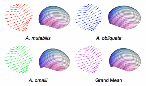
Figure 4. Mean shapes for each of the species-specific datasets and the grand mean for the pooled dataset as a while. The grand mean controls placement of the tangent plane onto which specimen surface shape configurations are projected in subsequent Procrustes PCA analysis.
Figure 4 summarizes the form of the mean shapes of each species, and the grand mean shape, for both the coordinate data and the surface models created from the coordinate data. Obviously the 15-grid level of resolution captures aspects of the valve vault, escutcheon, and beak morphology primarily. While this sampling scheme does not exhaust all the morphological variation available in these shells, inspection of the species-specific mean shapes resulting from its application indicates that this level of spatial sampling resolution does capture distinctions between the species. Let’s see if we can use these distinctions to develop a morphometric procedure for testing the degree of shape distinction that characterizes the shells of these species and (perhaps) for allocating unknown Astarte shells to the correct taxonomic group.
The first step toward realizing this goal is to use the Procrustes PCA method to summarize the major aspects of shape variation existing in these data and reduce its dimensionality. Of these two, reduction of the system’s dimensionality is the more important goal for our analysis since the number of variables used to characterize our surfaces is so large (621) and our sample size so small (30). Characterization of the primary modes of variation in these data is a by-product of this dimensionality reduction step. Nonetheless, from systematic and evolutionary points of view it’s an interesting by-product.
| No. | Eigenvalues | % Variation | Cum. % Variation | No. | Eigenvalues | % Variation | Cum. % Variation |
|---|---|---|---|---|---|---|---|
| 1 | 0.000924 | 36.830 | 36.830 | 15 | 0.000014 | 0.553 | 96.735 |
| 2 | 0.000508 | 20.246 | 57.076 | 16 | 0.000012 | 0.463 | 97.198 |
| 3 | 0.000315 | 12.540 | 69.616 | 17 | 0.000010 | 0.418 | 97.615 |
| 4 | 0.000176 | 7.031 | 76.647 | 18 | 0.000009 | 0.358 | 97.973 |
| 5 | 0.000135 | 5.384 | 82.031 | 19 | 0.000009 | 0.348 | 98.321 |
| 6 | 0.000092 | 3.670 | 85.702 | 20 | 0.000007 | 0.291 | 98.612 |
| 7 | 0.000054 | 2.151 | 87.853 | 21 | 0.000006 | 0.257 | 98.869 |
| 8 | 0.000049 | 1.943 | 89.786 | 22 | 0.000005 | 0.203 | 99.072 |
| 9 | 0.000045 | 1.809 | 91.606 | 23 | 0.000005 | 0.179 | 99.251 |
| 10 | 0.000031 | 1.249 | 92.855 | 24 | 0.000004 | 0.160 | 99.412 |
| 11 | 0.000027 | 1.093 | 93.948 | 25 | 0.000004 | 0.150 | 99.562 |
| 12 | 0.000023 | 0.918 | 94.866 | 26 | 0.000003 | 0.134 | 99.696 |
| 13 | 0.000017 | 0.690 | 95.557 | 27 | 0.000003 | 0.118 | 99.814 |
| 14 | 0.000016 | 0.625 | 96.182 | 28 | 0.000003 | 0.105 | 100.000 |
Eigenanalytic decomposition of the shape covariance matrix calculated from the pooled sample yields 28 positive eigenvalues (Table 2). Of these, 13 eigenvectors are required to capture 95 percent of the observed surface shape variation. This is impressive dimensionality reduction (97.8 percent) and pulls the number of variables necessary for the subsequent discriminant analysis back into the range of appropriateness given our sample size. A question might be raised concerning stability of eigenvectors calculated in such a high-dimensional space using so few data. But all we’re interested in at the moment is whether we can devise a discriminant space that separates these specimens from each other. In this sense we’re using Procrustes PCA as a data-transformation procedure to pack the surface variation signal recorded by these semilandmark data into the smallest number of variables possible and, at the same time, ensure those variables’ independence from one another.
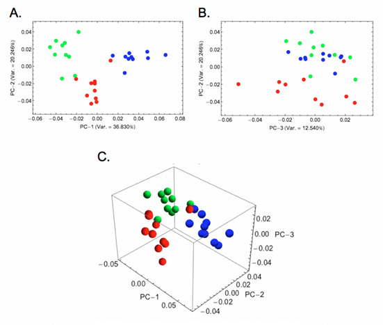
Figure 5. Ordination of Astarte surface shapes along the first three Procrustes PCA axes. Red symbols, A. mutabilis; Blue symbols A. obliquata; Green symbols A. omalii. A. The PC-1 - PC-2 subspace. B. The PC-3 - PC-2 subspace. C. The PC-1 - PC - 2 - PC-3 subspace.
While we’re not really that interested in the ordination of valve surfaces in the Procrustes PCA shape space per se, inspecting them is instructive (Fig. 5). Despite the fact that PC-1 - PC-2 subspace represents only slightly more than 50 percent of the observed shape variation, the distribution of valve surface geometries in this space suggest these species are distinct from one another in terms of those aspects of valve-surface variation captured by the 15-grid eigensurface sampling scheme. This ordination also suggests that species-specific differences in valve surface shape are largely responsible for the variation observed in the sample as a whole. Finally, there is a suggestion here that all three species are subequally distinct from each other with regard to valve vaulting, beak morphology, and escutcheon shape.
Many analysts would end their investigation here as a reasonable distinction between species was achieved in the PCA space. However, doing this would be tantamount to throwing away just under half the information on surface shape variation captured by the eigensurface measurement network and could result in an erroneous interpretation of the true level of distinction between these species that has been captured by these data. Remember, while it’s an easy matter to portray the ordinations of groups in the low dimensional PCA subspaces, these subspaces are neither optimized to distinguish between-groups variation, nor to present a complete picture of shape similarity relations, even within the PCA space. Rather such subspaces portray primary directions of variation within the pooled dataset and only represent the subset of biologically interesting patterns that happen to aligned with the dimensions plotted.
To create an accurate picture of group distinction we’ll need to run the projected positions of our Astarte surface shapes on all 13 of the Procrustes PCA axes that, together, account for 95 percent of observed shape variation into a CVA. This results in the specification of two discriminant axes since we’re trying to discriminate between three groups. More importantly though, the CVA technique will use all information residing on all 13 Procrustes PCA axes in its calculations, not just the first two or three that might be inspected as an intermediate step in data analysis. This is more information than we could reasonably hope to assimilate by looking at a series of scatterplots of shape distributions in 2D or 3D Procrustes PCA subspaces (e.g., Fig. 5) and should, at least in theory, result in an improved ordination. Since we’re only dealing with three groups, our CVA result will also have the convenient property of allowing us to portray all the information relevant to group discrimination that was picked up by our 15-grid eigensurface sampling scheme in a single 2D scatterplot (Fig. 6).
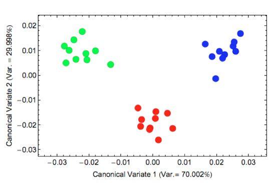
Figure 6. Ordination of the Procrustes PCA score data in the group difference-optimized canonical variates space. Symbols as in Fig. 5.
There really is no comparison between figures 5 and 6 in terms of the degree to which group distinctiveness is represented. Use of a method that’s designed to optimize the linear ordination space for group-differences, plus the addition of information from the ‘minor’ Procrustes PCA axes, has made a considerable difference. Through the application of a data analysis procedure capable of summarizing all the relevant valve surface shape information to optimize between-group differences we can (now) see that the specimens comprizing this sample are entirely distinct from one another in terms of their valve surface morphology, even in the gross manner captured by the 15-grid sampling scheme. Indeed, there’s a greater amount of between-groups distinction present on this plot than appears to be present in Plate 1. How can this be?
In Plate 1 we see the specimens comprizing our sample in their full glory, not only exhibiting the characteristics of their species, but also the iron stains, gouges, dings, scratches, that all fossils are heir to; even the occasional museum label. Many of these imperfections are substantial and would have been captured on the original 3D laser scans. However, the eigensurface interpolation procedure minimizes their effect by being blind to any that don’t affect the geometry of the surface morphology and by being effectively blind to those whose spatial dimensions fall below the resolution of the sampling grid. Moreover, the influence of any imperfections present in the grid data are minimized during the data analysis phase of the eigensurface procedure because these will tend to be aspects of shape variation peculiar to individual specimens, and so (most likely) located on the higher Procrustes PCA (= eigenvector) axes. Note that most of these axes were not carried forward and allowed to participate in the CVA. In effect, the eigensurface procedure tunes itself to emphasize the signals associated with the geometric regularities of morpho-group membership while rejecting the noise that characterizes individual specimens. This fine level of partitioning of the pattern of the morphological variation into generalized signal and idiosyncratic noise components is very difficult to achieve via simple qualitative inspection of specimen morphologies, in no small measure because the human visual system has been honed and refined over many millions of years to be drawn to the odd, the idiosyncratic, and the seemingly out of place (Broadbent 1958, Triesman 1982, Bertenfall 1992). In this sense eigensurface analysis — and other methods like it — not only extend the capabilities of the human visual system for assessing patterns within morphological data, it can be argued they represent substantial improvements on the human system.2
So, what do these Astarte discriminant axes ‘look like’ in terms of patterns of morphological variation? Table 3 illustrates the geometric character of the two Astarte discriminant axes using a series of theoretical surface shape configurations residing at equally spaced positions along each axis. These models were calculated using the method described in MacLeod (2009b).
| Axes | Modes | ||||
|---|---|---|---|---|---|
| 1 | 2 | 3 | 4 | 5 | |
| CV-1 |  (-0.028, 0.000) |  (-0.014, 0.000) |  (0.000, 0.000) |  (0.014, 0.000) |  (0.027, 0.000) |
| CV-2 |  (0.000, -0.026) |  (0.000, -0.015) |  (0.000, -0.004) |  (0.000, 0.007) |  (0.000, 0.018) |
Inspection of Table 3 shows that CV-1 captures the surface shape distinction between rather narrow forms characterized by (1) a high valve vault that verges strongly toward the beak; (2) a prominent, sharply pointed and asymmetrical beak; and (3) a long escutcheon oriented to form a decidedly shallow angle with the main portion of the valve periphery (low scores on CV-1), and broad forms characterized by (1) a low valve vault with a more equilateral vault curve; (2) a small, pointed and more symmetrical beak; and (3) a long escutcheon set at a much higher angle with regard to the valve periphery (high scores along CV-1). These models are consistent with the main taxonomic distinction shown along CV-1 which contrasts A. omalii (low scores) and A. obliquata (high scores). Similarly, CV-2 captures the distinction between forms with (1) a relatively high, equilaterally curved valve vault; (2) a small, pointed, asymmetrical beak; and (3) a relatively short escutcheon that meets the valve periphery at a relatively high angle (low scores on CV-2), with forms characterized by (1) a low, equilaterally curved valve vault; (2) a small, pointed, symmetrical beak; and (3) a relatively long escutcheon that meets the valve periphery at a relatively low angle (high scores on CV-2). These models are consistent with the main taxonomic distinction shown on by the scatter of shapes along CV-2 which contrasts A. mutabilis (low scores) and A. omalii - A. obliquata (high scores). In interpreting these modelling results it should be noted that the CV-2 models calculated for the higher values along this axis fall midway between the shape fields occupied by A. omalii and A. obliquata. Consequently these models reflect aspects of both species’ characteristic morphology, but correspond to no valve shapes that exist in the demonstration dataset.
The eigensurface technique is only one of a number of emerging morphometric methods that are now being developed to analyse 3D surfaces in the context of the geometric morphometric paradigm (see also Gunz et al. 2005 and Polly 2008). These procedures promise to extend the morphometric toolkit into the realm where image processing and analysis passes into virtual reality and computer vision. More pragmatically, their use has demonstrated that a previously unsuspected wealth of phylogenetic, taxonomic, functional, ecological, environmental and even behavioral information resides in the surface features of bones, shells and other structures, both living and fossil, as well as providing a means to analyse and extract that information from biological structures (e.g., Sievwright and MacLeod 2012). Indeed, application of this data sampling/analysis strategy even transcends biology itself (e.g., MacLeod et al. 2013) or, perhaps more properly, demonstrates that morphological data are ubiquitous across the biological and physical sciences while providing new tools that all scientists can use in a flexible and informative manner to probe, characterize, and discover the geometric patterns residing in natural phenomena.
Software for carrying out an eigensurface analysis is available as a set of MathematicaTM notebooks from myself. I’d like to acknowledge Jonathan Krieger for his work in helping to develop the algorithms on which the current implementation of eigensurface analysis is based.
Footnotes
1 Small holes in the specimen’s surface (e.g., entry of exit points for nerve chords in vertebrate crania) can be ignored.
2 See MacLeod et al. (2010) and Culverhouse et al. (in press) for more extended discussions of the limitations of human visual systems in the context of taxonomic analysis.
References
Bertenthal, B. I. 1992. Origins and early development of perception, action, and representation. Annual Review of Psychology, 47, 431–459.
Broadbent, D. E. 1958. Perception and communication. London, Pergamon.
CAMPBELL, N. A. and ATCHLEY, W. R. 1981. The geometry of canonical variate analysis. Systematic Zoology, 30, 268–280.
CULVERHOUSE, P. F., MACLEOD, N., WILLIAMS, R., BENFIELD, M., LOPES, R. and PICHERAL, M. in press. Is the consistency of taxonomic identifications a significant source of error in biodiversity and ecological investigations?: an empirical assessment. Marine Biology Research.
GUNZ, P., MITTEROECKER, P. and BOOKSTEIN, F. L. 2005. Semilandmarks in three dimensions. In D. E. Slice (ed). Modern Morphometrics in Physical Anthropology. Kluwer Academic/Plenum Publishers, New York, 73–98 pp.
MACLEOD, N. 1999. Generalizing and extending the eigenshape method of shape visualization and analysis. Paleobiology, 25, 107–138.
MACLEOD, N. 2007. Groups II. Palaeontological Association Newsletter, 65, 36–49.
MACLEOD, N. 2008. Understanding morphology in systematic contexts: 3D specimen ordination and 3D specimen recognition. In Q. Wheeler (ed). The New Taxonomy. CRC Press, Taylor & Francis Group, London, 143–210 pp.
MACLEOD, N. 2009a. Who is Procrustes and what has he done with my data? Palaeontological Association Newsletter, 70, 21–36.
MACLEOD, N. 2009b. Form & shape models. Palaeontological Association Newsletter, 72, 14–27.
MACLEOD, N. 2010a. Principal warps, relative warps and Procrustes PCA. Palaeontological Association Newsletter, 75, 22–33.
MACLEOD, N. 2010b. Shape models II: the thin plate spline. Palaeontological Association Newsletter, 73, 24–39.
MACLEOD, N. 2012. Going round the bend II: extended eigenshape analysis. Palaeontological Association Newsletter, 81, 23–39.
MACLEOD, N., KRIEGER, J. and JONES, K. E. 2013. Geometric morphometric approaches to acoustic signal analysis in mammalian biology. Hystrix, http://dx.doi.org/10.4404/hystrix-24.1-6299.
POLLY, P. D. 2008. Adaptive zones and the pinniped ankle: a 3D quantitative analysis of carnivoran tarsal evolution. In E. Sargis and M. Dagosto (eds). Mammalian Evolutionary Morphology: A Tribute to Frederick S. Szalay. Springer, Dordrecht, The Netherlands, 165–194 pp.
ROHLF, F. J. and SLICE, D. 1990. Extensions of the Procrustes method for optimal superposition of landmarks. Systematic Zoology, 39, 40–59.
SIEVWRIGHT, H. and MACLEOD, N. 2012. Eigensurface analysis, ecology, and modelling of morphological adaptation in the falconiform humerus (Falconiformes: Aves). Zoological Journal of the Linnean Society, 165, 390-415.
TREISMAN, A. 1982. Perceptual grouping and attention in visual search for features and for objects. Journal of Experimental Psychology Human Perception and Performance, 8, 194–214.
